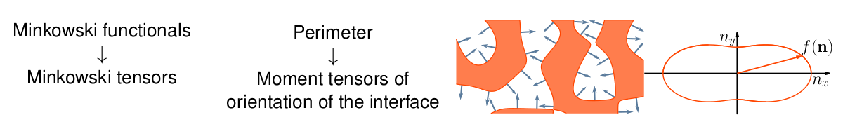
The Minkowski tensors can be intuitively defined via weighted volume or surface integrals in the Cartesian representation. In praticular, this definition is an intuitive generalization of the Minkowski scalars. For example, the perimeter can be generalized to the moment tensor of the orientation of the interface (surface area measure).
2D T-Inv Tensors
In two dimensions, the second-rank translation invariant (T-Inv) tensors are defined in the Cartesian representation as follows using the normal vector  on the boundary:


with  being the curvature and using the symmetric tensor product
  , which can be represented by a matrix
with the entry  in row
  and column
  .
.
Higher rank translation invariant (T-Inv) tensors


where  is the tensor product.
Relation to IMTs
These Cartesian Minkowski Tensors (CMT) and the Irreducible Minkowski Tensors (IMT) are, of course, only different representations of the same Minkowski tensors and can therefore be related to each other.
 ,
,
where  . Because all summands with
  vanish due to the vanishing the Fourier components of
  , we obtain

Note that the Fourier coefficients of are independent of the body  . For
. For  , they are given by

where  is the unit tensor,
  is the zero tensor, and the
  are Pauli matrices with
 and
and  .
.
Thus, the second-rank CMT  can be expressed by the IMTs
  ,
,  , and
, and  :
:

and vice versa:


Thus the Minkowski structure metric  can be expressed by the eigenvalues
  and
and  of the Minkowski tensor :
 .
.
Similarly the fourth rank index  can be expressed by the components of the Minkowski tensor
  , where for convenience the coordinate axes are assumed to coincide with the eigenvectors of :
 .
.
2D T-Cov Tensors
While the IMT offer an intuitive quantification of the degree of anisotropy for arbitrary ranks of the tensors, the Cartesian representation offers an intuitive definition of not only of the transliation-invariant (T-Inv) Minkowski tensors but also of the translation-covariant (T-Cov) tensors. The latter are required for a complete additive characterization (according to Alesker’s theorem).
Using the position vector  the Minkowski Vectors are defined as:


and the second-rank translation covariant (T-Cov) Minkowski tensors as:


 .
.
They thus generalize the area or perimeter to the second moment of the mass distribution of a solid or hollow body.
They thus contain the information of the tensor of inertia of such massive bodies.
The T-covariant tensors for short, depend on the chosen origin and transform as follows when the object K is being translated by a vector  :
:
 .
.
3D T-Inv and T-Cov Tensors
Second-rank T-Inv Minkowski Tensors


Minkowski Vectors


Second-rank T-Cov Minkowski Tensors


dD Tensors
Similar integrals can be defined for smooth bodies in arbitrary dimensions using the elementary symmetric function of the principal curvatures.