For sufficiently smooth bodies  , the Minkowski Functionals can be intuitively defined via (weighted) integrals over the volume or boundary of the body .
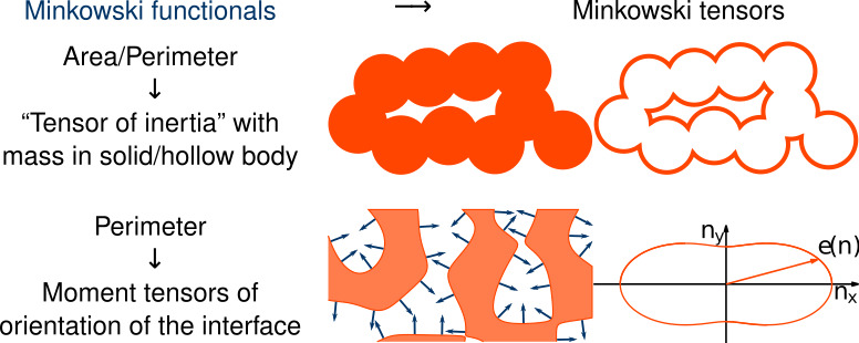
The scalar functionals can be interpreted as area, perimeter, or the Euler characteristic, which is a topological constant. The vectors are closely related to the centers of mass in either solid or hollow bodies. Accordingly, the second-rank tensors correspond the tensors of inertia, or they can be interpreted as the moment tensors of the distribution of the normals on the boundary.
Minkowski Functionals
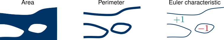
Area

Perimeter

Euler characteristic

with
 = curvature
Cartesian representation (Minkowski Tensors)
Using the position vector  and the normal vector
  on the boundary, the Minkowski Vectors can be defined in the Cartesian representation.
The second-rank Minkowski tensors are defined using the symmetric tensor product  .
.
Minkowski Vectors


Minkowski Tensors


Irreducible representation (Circular Minkowski Tensors)
Due to the different rotational symmetries of, for example, a rectangle and a triangle, their anisotropy is encoded in Minkowski tensors of different rank, for example, in  for the rectangle and in
  for the triangle. To define rotational invariants that quantify the degree of anisotropy of different ranks (different rotational symmetries), we need the irreducible representation. Loosely speaking, it is a decomposition into tensors with an
  -fold rotational symmetries.
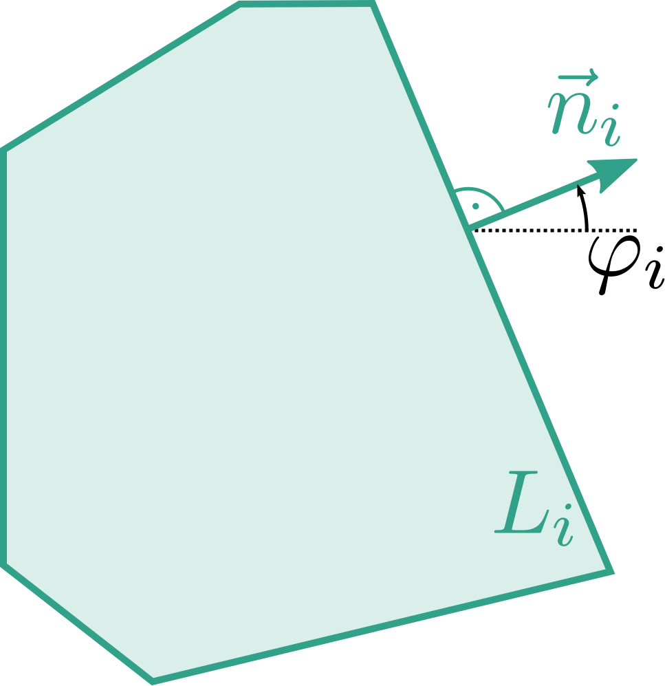
Consider a polygon with edge lengths  :
:
 .
.
Density of normals:

Fourier analysis:

The zeroth Fourier component is the circumference of the polygon: 
The first Fourier component vanishes for all closed polygons: 
The shape indices  are defined as
(1) 
 for
for  vanish only for the circle (left). If there is only a single anisotropy index non-zero, the choice of this rank defines a convex shapes with an -fold rotational symmetry.

 for closed polygons.
 is the quadrupole component of the normal density, it is related to
 can detect anisotropy in a three-fold symmetric system (e.g. suitable for detecting equilateral triangles)
 can detect anisotropy in a four-fold symmetric system (e.g. suitable for detecting rectangles)
 …
…
Morphometric distance
A morphometric distance of a polygon to a reference structure  can be quantified by considering the pseudo distance function
![d(K) = \sqrt{\sum\limits_l [q_l(K) - q_l(R)]^2}](https://morphometry.org/wp-content/ql-cache/quicklatex.com-cf3d48b1bdf7af5f5f7c53d7b6ad61c5_l3.png "Rendered by QuickLaTeX.com") .
.