Anisotropy analysis by IMT – morphometry.org

Irreducible Minkowski Tensors (IMTs) provide a systematic, robust and quantitative characterization of shapes. For this introduction, we focus on 2D shapes that are convex sets, even though the anisotropy analysis remains useful for non-convex structures. We will also assume that the shape has a (piecewise) smooth contour, like a polygon for instance. Finally, we focus on the translation-invariant tensors, which are most commonly used. (For people already familiar with Cartesian Minkowski tensors, the IMTs discussed here are an alternative representation of the $W_1^{0,s}$ tensors. The 3D version of Irreducible Minkowski Tensors is described here.)

Irreducible Minkowski Tensors (IMT)

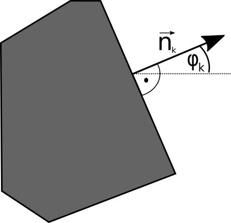
Irreducible Minkowski Tensors quantify the geometry of the interface of a shape. The lowest order is the perimeter, i.e. the length of the boundary of the shape. Higher orders quantify the deviation of a shape’s boundary from perfect isotropy (i.e., a circle in 2D, or a sphere in 3D). For simplicity, let us consider a polygonal shape:

Here $L_k$ is the lengths of the $k$ -th edge, and $\vec n_k$ is the outer normal vector of the $k$ -th edge. Moreover, we define the vectors,

$\vec L_k = L_k \vec n_k$ .

Note that the vectors $L_k$ are just the edges of the polygon, rotated by 90 degrees. It is useful to realize that a convex polygon can be uniquely reconstructed if we know the set of vectors $\{ \vec L_k \}$ : We simply concatenate the vectors $L_k$ , sorted by the angle they span with the $x$ axis, and obtain a copy of the original polygon, rotated by 90 degrees:

Because the sorted the vectors by their polar angle, the reconstructed shape is convex. (Clearly, the mapping between polygons and their set of vectors $\{L_k\}$ is only one-to-one if and only if the polygon was convex in the first place.)

We now define the normal density as the function

$\rho_K(\varphi) = \sum\limits_k L_k \, \delta(\varphi-\varphi_k)$

where $\delta$ is Dirac’s delta distribution:

The function $\rho_K$ characterizes the interface of the shape $K$ . (The function $\rho_K$ is sometimes referred to as the extended Gaussian image, or EGI).
This function is degenerate in our case (it consists only of Dirac $\delta$ ‘s) because we analyzed a polygonal object. If the shape’s interface had had smooth curved parts, the normal density function would have featured a smooth component as well (we will find examples below).

Minkowski analysis

The key idea of IMTs is to decompose the normal density into the irreducible representations of the rotation group. In two dimensions, this is merely the well-known Fourier series of a $2\pi$ -periodic function $\rho_K$ ,

$\psi_s(K) = \int\limits_{0}^{2\pi} \textnormal d \varphi \,\exp(\I s \varphi) \, \rho_K(\varphi) = \sum\limits_{k=-\infty}^{\infty} L_k \, \exp(\I s \varphi_k)$ .

The complex numbers $\psi_s(K)$ are the Irreducible Minkowski Tensors. Knowing all $\psi_s$ (all Fourier coefficients), we can reconstruct the function $\rho_K(\phi)$ , and thus, the convex shape $K$ we started with. Because the $\psi_s$ are the Fourier coefficients of a real function, they obey the Hermitian symmetry, $\psi_{-s} = \psi^*_s$ . The zeroth coefficient is precisely the perimeter of the shape, $\psi_0(K) = P(K)$ . For any closed contour, we saw above that the vectors $\vec L_k$ sum to zero. This has the consequence that $\psi_{\pm 1} = 0$ . Any higher IMTs contain shape information about the anisotropic nature of the contour.

Loosely speaking, the $\psi_s$ tensor described the component of the interface with $s$ -fold, but not higher, symmetry. The shape information contained in the various $\psi_s$ , $s\geq 2$ , is disjoint: For example, $\psi_3$ contains the 3-fold part, but not the 6-fold, 9-fold symmetric part of $\rho_K$ . For example, $\psi_2$ is the quadrupole component of the normal density, and $\psi_0$ , again, is the monopole part (the perimeter of the shape). Closed contours cannot have a dipole part, thus $\psi_{\pm1} = 0$ .

Minkowski synthesis

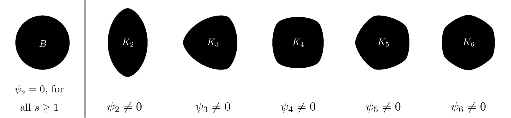
The mapping between convex shapes $K$ and their set of IMTs $\{\psi_s(K)\}$ is bijective, i.e., every sufficiently smooth shape has a unique function $\normaldensity_K$ , and thus Fourier coefficients $\psi_s(K)$ . Conversely, there is at most one convex shape for a prescribed set of IMTs: Via the Fourier series, we can reconstruct the function $\rho_K$ from the coefficients $\psi_s$ , and if $\rho_K$ is a non-negative function, then it defines a unique convex shape with that normal density (“Minkowski synthesis”; this is the solution of the Minkowski problem). This is how we have generated the following image:

Only for the ball all IMTs $\psi_s$ with $s\geq1$ vanish (left). If there is a single Fourier component $\psi_n$ non-zero, the choice of $n$ defines a convex shapes with an $n$ -fold rotational symmetry.

These shapes $K_n$ are characterized by a particular $\psi_s$ , i.e., all coefficients vanish $\psi_s=0$ , save for $\psi_0$ , and $\psi_{\pm n}$ . Their normal density function is a pure sine wave offset such that it is nonnegative, $\rho_{K_n}(\varphi) = 1 + \cos(n\varphi)$ . (One could term the football shape $K_2$ the “ideal quadrupole” in that it only features a quadrupole component in its normal density. The tensor $\psi_2$ is connected to the well-known Cartesian Minkowski Tensor $W_1^{0,2}$ .)

Examples

Clearly, the $s$ -th irreducible Minkowski tensor is connected with an $s$ -fold rotational symmetry. We note that the shapes in the previous image are smooth objects (save for the $n$ pointy tips), because their normal density is a pure sine wave. To construct regular polygons, higher-order Fourier modes must be added. For example, a regular triangle $\Delta$ with unit sides features nonzero IMTs $\psi_3, \psi_6, \psi_9, \dotsc$ :

$\rho_\Delta = \delta(\varphi) + \delta(\varphi-2\pi/3) + \delta(\varphi-4\pi/3)$

$\psi_{3n}(\Delta) = 1 + \exp(\I \cdot 3n\cdot \frac{2\pi}{3}) + \exp(\I \cdot 3n\cdot \frac{4\pi}{3}) = 3$

$\psi_{3n+1}(\Delta) = \psi_{3n+2}(\Delta) = 0$ .

The unit ball $B$ has the normal density $\rho_B(\phi) = 1$ and is perfectly isotropic. Consequently, we find that the perimeter is $\psi_0 = 2\pi$ , and all other IMTs $\psi_s = 0$ .

Behavior under Transformations

Rotations

Rotating a shape $K$ in the plane amounts to shifting the function $\rho_K(\varphi) \to \rho_K(\varphi - \theta)$ , that is, a shift of the complex phases of all $\psi_s(K)$ . More precisely, a counterclockwise rotation by angle $\theta$ modifies the IMTs

$\psi_s(K) \to \psi_s(\hat R(\theta) K) = \psi_s(K) \exp(\I s\theta)$

Here $\hat R$ is the operator that rotates a shape by the given angle.

Translations and scalings

Translating the shape $K$ in the plane does not modify the IMTs; they are translation-invariant. Scaling by a linear factor $\lambda$ changes the IMTs by a factor $\lambda$ as well; they are of homogeneity 1, as the perimeter.

$\psi_s(\vec x + K) = \psi_s(K)$ ,

$\psi_s(\lambda K) = \lambda \psi_s(K)$ .

Minkowski Structure Metrics q_s

Frequently, the orientation and size of an object is not of interest, and a metric invariant under rotation, scaling, and translation is required. This is provided by the Minkowski Structure Metrics (MSMs) $q_s$ . These shape indices are defined as

$q_s(K) := \frac{|\psi_s(K)|}{\psi_0(K)}$ .

The $q_s$ are invariant under rigid motions (rotation and translation) and scaling of $K$ .

$q_s$ detects the presence of $s$ -fold-symmetric component in the normal density.
For example, $q_2$ is sensitive to the quadrupole component, and is sensitive to rod-like shapes. $q_3$ can be used to find shapes with predominantly threefold symmetry, such as equilateral triangles. $q_6$ is used to detect regular hexagons, and to find hexagonal order in 2D packings (in this application the IMTs are a refinement of Steinhardt’s bond-orientational order parameters [bibcite key=mickel2013shortcomings]).

The $q_s$ are fingerprints of a particular class of shapes, and blind to rotation and scaling. The $q_s$ may thus be used to classify shapes, ignoring their size and orientation.

Distinguished directions

Each of Minkowski tensor of rank $s$ distinguishes $s$ spatial directions. These are the directions in which “most” of the interface is oriented. We can calculate the preferred directions of a body $K$ from its Minkowski tensor $\psi_s(K)$ via the complex argument of $\psi_s$ :

direction angle = $\frac{\textnormal{arg}(\psi_s(K)) + 2 \pi n}{s}$ for $n = 0, ..., s-1$

Specifically for $\psi_2$ , the quadrupole, the distinguished directions are the antipodal vectors with the direction angles

$\tfrac 12 \textnormal{arg}(\psi_s(K))$ and $\tfrac 12 \textnormal{arg}(\psi_s(K)) + \pi$

For an interactive illustration, see morphometer.