Point processes – morphometry.org

Point processes are random collections of points [bibcite key=last2017lectures]. They can model a huge variety of complex, amorphous systems from science to technology, including particles in physical systems, galaxy clusters in the universe, trees in forest, and nodes in telecommunication networks [bibcite key=chiu2013stochastic,illian2008statistical].

Any given point pattern defines a partition (or “quantization”) of the Euclidean space, the so-called Voronoi tessellation. The Voronoi cell $C_i$ of a point $\vec{z}_i$ in the point pattern consists of all sites in space that are closer to $\vec{z}_i$ than to any other points $\vec{z}_{j\neq i}$ in the point pattern. The dual of the Voronoi tessellation is the Delaunay triangulation, for which no point is the interior of the circumradius of any triangle.

The Minkowski functionals and tensors can quantify the structure of these tessellation, for example, they can detect strong volume fluctuations or the formation of small crystallites in the point pattern [bibcite key=klatt2017cell,kapfer2012jammed]. Examples are presented in the morphometer (2D online tool). The point processes included in the morphometer are explained in the following.

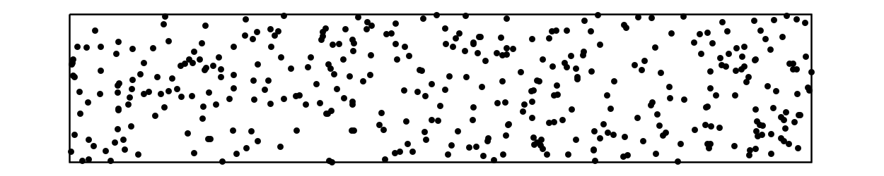
N random points — The Binomial Point Processes

$N$ independent points are uniformly distributed in the observation area. The result is a binomial point process of $N$ points.

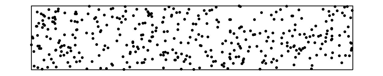
The Ideal Gas — The Poisson Point Processes (Poisson)

A Poisson point process is, intuitively speaking, a completely independent point process [bibcite key=last2017lectures]. The points are randomly placed in space uniformly distributed. The number of points inside the observation window follows a Poisson distribution. The coordinates of the points are uniformly distributed in the simulation box and mutually independent from each other. The Poisson point process can be interpreted as a snapshot of the ideal gas of non-interacting particles in the grand-canonical ensemble, where the intensity of the Poisson point process is equivalent to the fugacity of the ideal gas (if the unit of length is defined by the thermal de Broglie wavelength).

If a fixed number of random points are independently and uniformly distributed in the observation window (like when adding random points in the 2D online tool), the resulting point pattern is the realization of a Binomial point process [bibcite key=chiu2013stochastic]. In the thermodynamic limit (where the mean number of points per volume is fixed but the volume diverges), the Binomial point process represents snapshots of the ideal gas in the canonical ensemble.

The Thomas Point Process (Poisson Cluster)

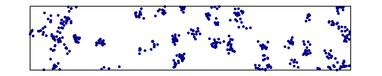
Poisson cluster processes are also known as centre-satellite processes. They are examples of clustering Neyman-Scott processes [bibcite key=chiu2013stochastic,illian2008statistical].

Starting from a realization of a homogeneous Poisson point process, each of the points defines the center of cluster (and is therefore called “parent point”; therefore the intensity of the Poisson point process is denoted by $\rho_p$ ).

The clusters, which are centered at the parent points, are independently and identically distributed. The number of points in each cluster is a random number with mean value $\bar{c}$ . The final point process includes only the children and not the parents (the latter only serve as the centers of the clusters). Because of the statistical independence, the intensity of the Neyman-Scott process is given by $\rho = \rho_p\bar{c}$ .

Here we simulate a (modified) Thomas process, where the number of points in a cluster follows a Poisson distribution. The displacement of each child from its parent follows the isotropic $d$ -dimensional Gaussian distribution with variance $\sigma^2$ . The “degree of clustering'” in the model is controlled by the parameters $\bar{c}$ and $\sigma$ .

To simulate the Thomas process in our simulation box $[0,L)^2$ , we first draw the number of parent points from a Poisson distribution with mean value $\lambda_pL^2$ . The parent points are uniformly distributed in $[0,L)^2$ . The number of children is drawn (for each parent point separately) from a Poisson distribution with mean value $\bar{c}$ . Finally, the coordinates of the children are sampled from the corresponding Gaussian distribution.

Random sequential addition for Hard Disks — Matérn III Process (RSA)

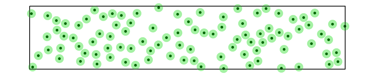
This model is also known as “random sequential addition”, “simple sequential inhibition”, or “Poisson disc sampling”. An important application is the irreversible adsorption or adhesion of proteins or cells at solid interfaces [bibcite key=talbot2000from], where a particle diffuses above a surface until it tries to attach to the surface at a random site. If it sticks to the surface, it can no longer move. Therefore, it blocks the adsorptions of other particles in its neighborhood.

In the mathematical model discs are subsequently placed on a surface. They are randomly and sequentially inserted into the simulation box (with random coordinates), but they are only accepted if such that they do not overlap with discs that were inserted previously. Once inserted, the discs can no longer change their positions. The process terminates when there is no space left for new disks. The packing becomes saturated.

In the mathematics literature, this is known as the saturation limit of the Matérn III process [bibcite key=chiu2013stochastic]. In 2D, the packing fraction, that is, the fraction of space covered by the spheres, can reach 54.7% [bibcite key=zhang2013precise].

In the 2D tool, we actually do not simulate this limit but abort the simulation once we reach a chosen packing fraction.

The Hyperplane Intersection Process (HIP)

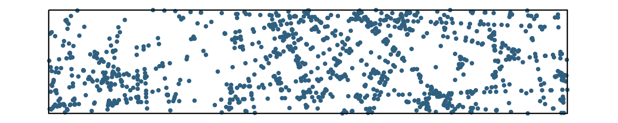
The process is based on the so-called Poisson line tessellation, which is–intuitively speaking–a collection of mutually independent lines that are randomly oriented and uniformly distributed in space [bibcite key=schneider2008stochastic]. More precisely, the number of lines that intersect a disc follows a Poisson distribution, and the distance between the origin and a line that intersects the disc is uniformly distributed between zero and the radius of the disc. These properties directly define a simple simulation procedure.

The points in the realization of a “lines intersection process” are then obtained by the intersections of two lines. It is a strongly clustering point process, in that the pair correlation function $g_2(r)$ diverges for $r\rightarrow 0$ ; for an analytic expression of $g_2(r)$ , see [bibcite key=heinrich2006central].

Because a line spans the whole plane, it induces infinitely long-ranged correlations, which increase the density fluctuations. The process exhibits correlations on large length scales that increase the density fluctuations in the system. The lines intersection process is therefore fluctuating qualitatively stronger than a completely random Poisson point process. The variance of the number of points in a $d$ -dimensional spherical observation window of radius $R$ grows like $R^{2d-1}$ , that is, faster than the volume of the observation window (for $d>1$ ) [bibcite key=heinrich2006central]. It is therefore a prototypical example of a “hyperfluctuating” point process (the opposite of a hyperuniform point process [bibcite key=torquato2003local]), that is, there are arbitrary long-range spatial density fluctuations ( $\infty$ in an $\infty$ system).

The Permanental Point Process (Permanental)

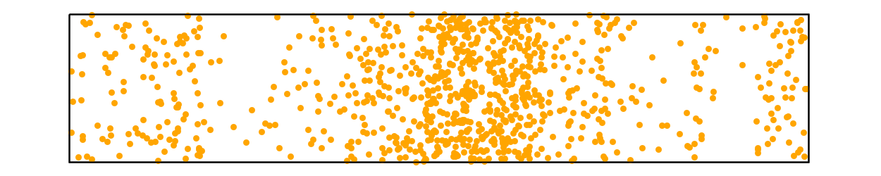
Permanental point processes can model the positions of bosons. Their realizations form clustering point patterns (in contrast to the repulsive determinantal point processes, which model fermions) [bibcite key=hough2006determinantal].

Mathematically speaking, it is defined via its $n$ -point correlation functions that are based on permutations and a kernel $K:\mathbb{R}^d\times\mathbb{R}^d \rightarrow \mathbb{R}$ [bibcite key=last2017lectures,mccullagh2006permanental]:

$g_n(x_1,\ldots,x_n) = \rho^{-n}\mathrm{per}\left(K(x_i,x_j)\right)_{1\leq i,j \leq n} = \rho^{-n}\sum_{\sigma\in\Sigma_n}\prod_{i=1}^{n}K(x_i,x_{\sigma(i)}),$

where $\Sigma_n$ denotes the group of permutations $\sigma$ of $\{1,\ldots,n\}$ .

The permanental process simulated in the 2D online tool has the intuitive interpretation of a doubly stochastic Poisson proces: first, we simulate a random density profile function, which is then used as the intesity function of an inhomogeneous Poisson point process [bibcite key=last2017lectures].

This is still a huge class of processes, from which we have chosen random intensity functions that are defined by the sum of the absolute values of two realizations of a so-called Gaussian random waves model. The latter is given by the superposition of plane waves with a constant wavenumber $q$ but with random phases and orientations of the wave vectors. By choosing an anisotropic orientation distribution for the wave vectors, a point pattern that is strongly anisotropic can be created. In the morphometer the angle between the wave vector and the $y$ -axis is uniformly distributed in the interval $[-\omega,\omega)$ .

For more details, see Section 13.2.2.3 in [bibcite key=klatt2017cell] (where $q$ is denoted by $k_i$ and $\theta$ by $\omega$ ).

[/bibshow]